Bild einlesen und anzeigen mithilfe von Scikit-Image
from skimage.io import imread
import numpy as np
import matplotlib.pyplot as plt
def default_show(image, title=None):
"""
Displays an image using matplotlib.
Parameters:
- image: The image to be displayed.
- title: Optional title for the plot.
"""
plt.figure(figsize=(10, 10)) # Set the figure size to be big
plt.imshow(image, cmap='gray')
if title:
plt.title(title)
plt.axis('off')
plt.show()image = imread('sea_wall.jpg')
# showing the image
default_show(image, "Sea Wall")
# printing the type and data of the image
print("Datentyp:", image.dtype)
print("Shape:", image.shape)
print("Dimensionen:", image.ndim)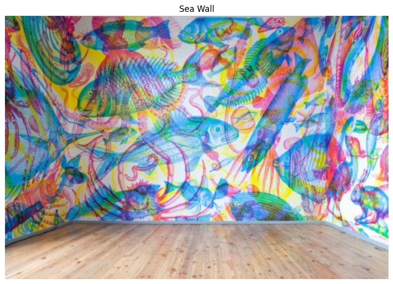
Datentyp: uint8
Shape: (322, 468, 3)
Dimensionen: 3
Das eingelesene Bild ist ein NumPy-Array mit dem Datentyp uint8, d. h. jedes Pixel kann Werte von 0 bis 255 annehmen.
Der Aufbau des Arrays ist dreidimensional mit der Struktur (Höhe, Breite, Kanäle). Ein Farbbild hat typischerweise 3 Kanäle (RGB), also z. B. image.shape = (512, 768, 3).
Jeder Pixel besteht aus drei Werten: Rot, Grün und Blau.
Zugriff auf den roten Kanal eines Pixels z. B. über image[y, x, 0].
Drei Farbkanäle des Bildes getrennt
def read_red_channel(image):
    """
    Function to read the red channel of an image
    :param image: input image
    :return: red channel of the image
    """
    # Extracting the red channel
    red_channel = image[:, :, 0]
    return red_channel

def read_green_channel(image):
    """
    Function to read the green channel of an image
    :param image: input image
    :return: green channel of the image
    """
    # Extracting the green channel
    green_channel = image[:, :, 1]
    return green_channel

def read_blue_channel(image):
    """
    Function to read the blue channel of an image
    :param image: input image
    :return: blue channel of the image
    """
    # Extracting the blue channel
    blue_channel = image[:, :, 2]
    return blue_channel
# Show each color channel separately
images = ['hidden.png', 'sea_wall.jpg', 'wood.jpg']
fig, axes = plt.subplots(3, 3, figsize=(15, 10))
for i, img_path in enumerate(images):
img = imread(img_path)
axes[i, 0].imshow(read_red_channel(img), cmap='Reds')
axes[i, 0].set_title(f"{img_path} - Red")
axes[i, 1].imshow(read_green_channel(img), cmap='Greens')
axes[i, 1].set_title(f"{img_path} - Green")
axes[i, 2].imshow(read_blue_channel(img), cmap='Blues')
axes[i, 2].set_title(f"{img_path} - Blue")
plt.tight_layout()
plt.show()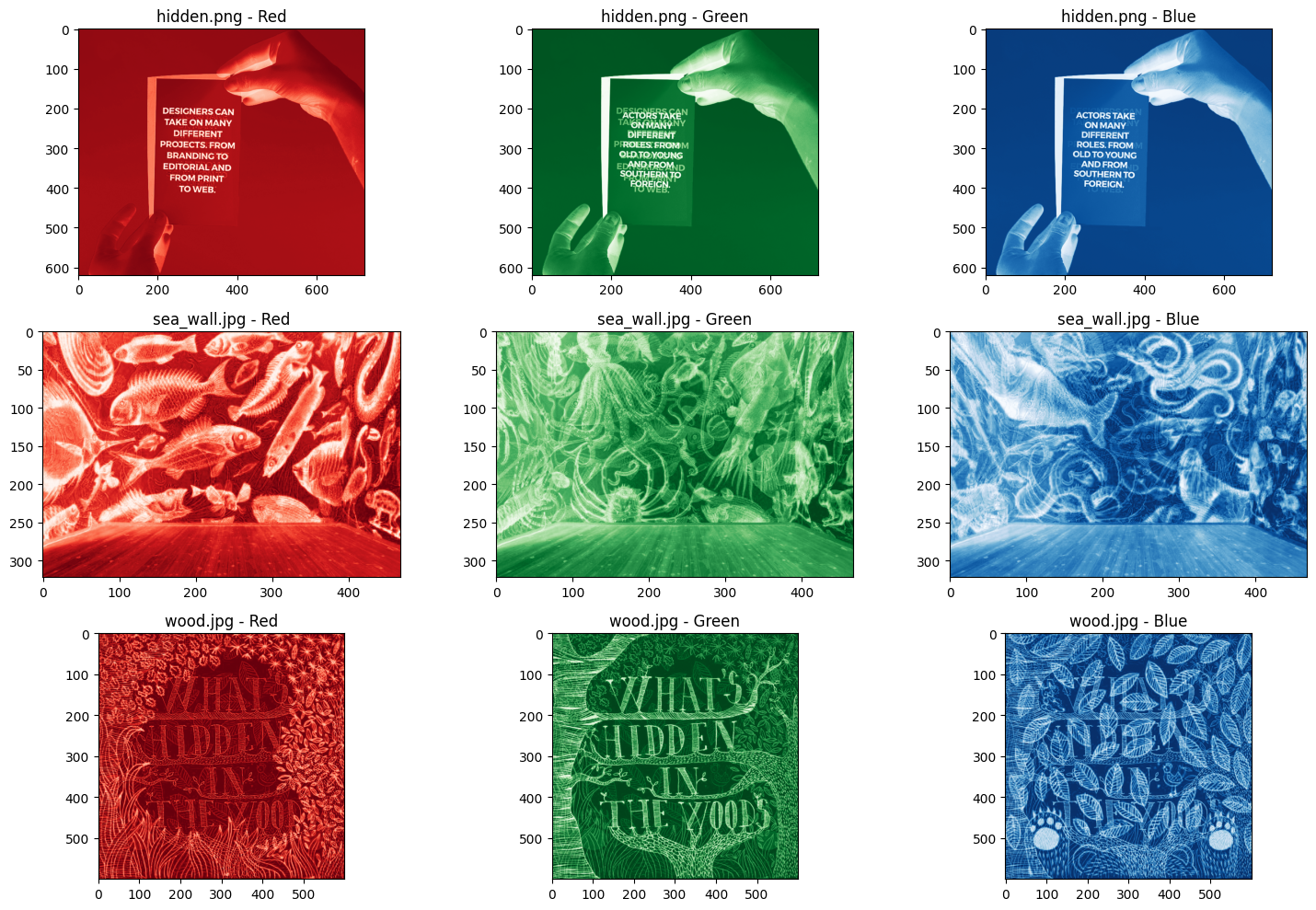
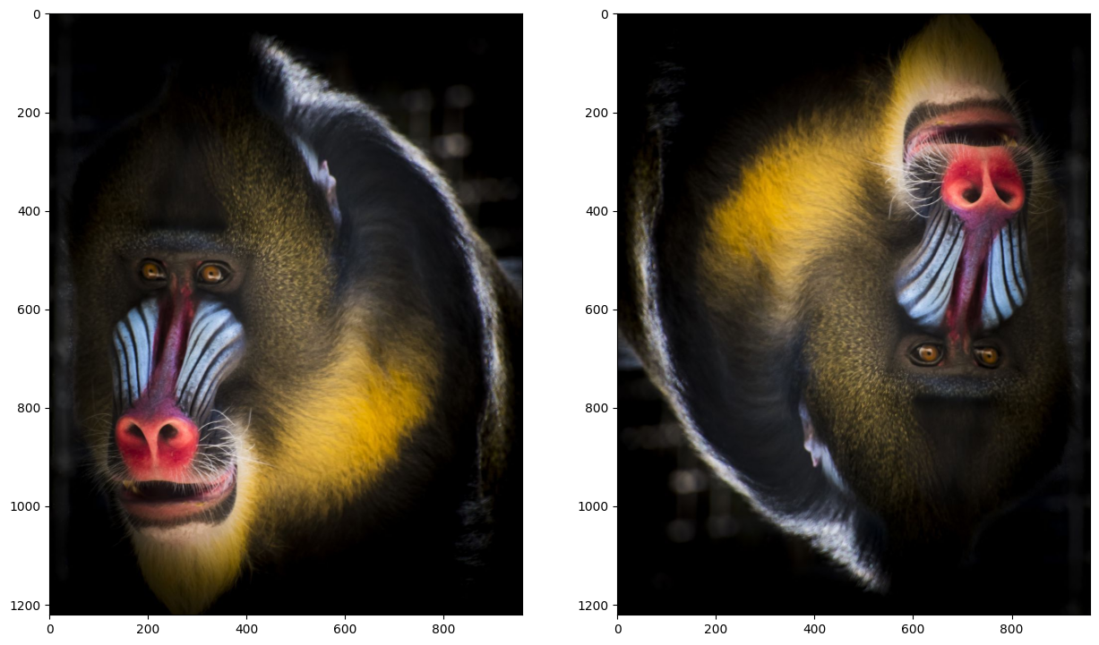
def invert_horizontal(image):
    return [row[::-1] for row in image]

def invert_vertical(image):
    return image[::-1]
image = imread('monkey.jpg')
plt.figure(figsize=(15, 10))
plt.subplot(121)
plt.imshow(invert_horizontal(image))
plt.subplot(122)
plt.imshow(invert_vertical(image))<matplotlib.image.AxesImage at 0x1473084a850>
def computeHisto(image):
    histo = np.zeros(256, dtype=int)

    height, width = image.shape

    # Gehe alle Pixel durch und zähle Häufigkeiten
    for y in range(height):
        for x in range(width):
            intensity = image[y, x]
            histo[intensity] += 1

return histofig, axes = plt.subplots(2, 3, figsize=(20, 10)) # Create a 2x3 grid of subplots
# Process images from bild01.jpg to bild05.jpg
for i in range(1, 6):
grayscale_image = imread(f'bild0{i}.jpg', as_gray=True) # Read image in grayscale
grayscale_image = (grayscale_image * 255).astype(np.uint8) # Convert to uint8
histo = computeHisto(grayscale_image) # Compute histogram
# Display histogram in subplot
row, col = divmod(i - 1, 3) # Calculate row and column indices
axes[row, col].bar(range(256), histo, width=1, color='gray')
axes[row, col].set_title(f"bild0{i}.jpg")
axes[row, col].set_xlabel("Intensitätsstufen")
axes[row, col].set_ylabel("Anzahl der Pixel")
# Hide the unused subplot
axes[1, 2].axis('off')
plt.tight_layout()
plt.show()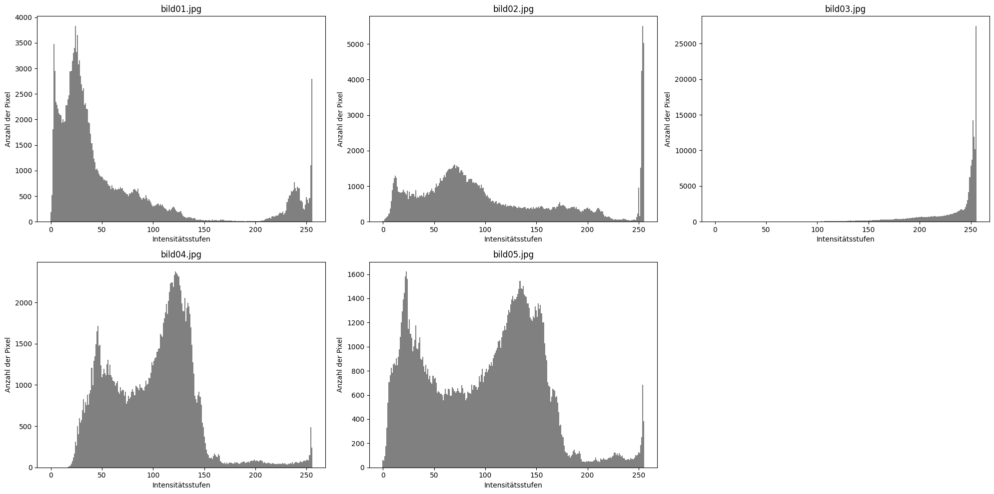
a) Welche Aufnahmefehler sind in 01 und 03 zu erkennen? Woran ist dies im Histogramm erkennbar?
-
Bild01:
Fehler: Bild ist unterbelichtet (zu dunkel). Die Pixelwerte sind stark im dunklen Bereich (nahe 0) konzentriert. Es gibt fast keine hohen Helligkeitswerte. -
Bild03:
Fehler: Kein echter Fehler – Bild ist gut belichtet. Die Helligkeitswerte sind über den gesamten Bereich (0–255) gleichmäßig verteilt → kein Kontrastverlust, keine Unter-/Überbelichtung.
b) Bild01 ist das aufgenommene Bild. Bild02 wurde nachbearbeitet. Die Helligkeit wurde erhöht. Woran ist dies im Histogramm erkennbar? Welche Daten gehen dabei verloren?
Pixel, die in Bild01 bereits nah an 255 lagen, sind beim Helligkeitsschub “übergelaufen” und wurden auf 255 gekappt.
Dadurch gehen Helligkeitsunterschiede in den hellen Bereichen verloren → Details sind abgeschnitten (Clipping).
c) Bild04 ist das aufgenommene Bild. Bild05 wurde einem Bearbeitungsschritt unterzogen. Was wurde in Bild05 verändert? Woran kann man dies in seinem Histogramm erkennen?
Das Histogramm von Bild05 hat nur wenige schmale Peaks (z. B. bei 0, 128, 255), der Rest ist leer.
Das bedeutet: Es gibt nur noch ganz bestimmte Intensitätswerte → typische Folge von Posterisierung oder Farb-/Graustufenumwandlung mit geringer Bit-Tiefe.
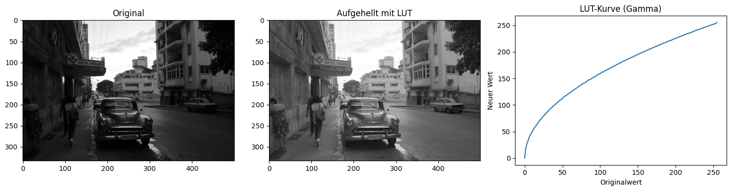
def create_lut_brighten():
    """
    Erzeugt eine Lookup-Tabelle, die dunkle Bereiche aufhellt,
    ohne helle Bereiche stark zu verändern.
    → z. B. mit einer Gammakorrektur (gamma < 1)
    """
    gamma = 0.5  # Geringer als 1 → Aufhellung dunkler Bereiche
    lut = np.array([int(255 * ((i / 255) ** gamma)) for i in range(256)], dtype=np.uint8)
    return lut
def apply_lut(image, lut):
"""
Wendet eine Lookup-Tabelle auf ein Graustufenbild an.
image: 2D NumPy-Array
lut: 1D NumPy-Array mit 256 Einträgen
"""
height, width = image.shape
output = np.zeros_like(image)
for y in range(height):
for x in range(width):
output[y, x] = lut[image[y, x]]
return output# Bild laden (zuvor in Graustufen umgewandelt)
image = imread("Bild01.jpg", as_gray=True)
image = (image * 255).astype(np.uint8)
lut = create_lut_brighten()
brightened = apply_lut(image, lut)
# Plot
plt.figure(figsize=(15, 4))
plt.subplot(1, 3, 1)
plt.imshow(image, cmap='gray')
plt.title("Original")
plt.subplot(1, 3, 2)
plt.imshow(brightened, cmap='gray')
plt.title("Aufgehellt mit LUT")
plt.subplot(1, 3, 3)
plt.plot(lut)
plt.title("LUT-Kurve (Gamma)")
plt.xlabel("Originalwert")
plt.ylabel("Neuer Wert")
plt.tight_layout()
plt.show()